SimTrack3D: Monocular 3D Trajectory Prediction of Fast-Moving Shuttlecocks via Broadcast-Calibrated Sim-to-Real Transfer
Project page · 2026
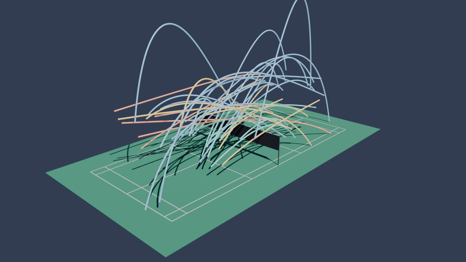
Demo
Abstract
Recovering metric 3D trajectories of fast-moving sports projectiles from a single uncalibrated broadcast camera is fundamentally ill-posed. In broadcast badminton, standard monocular depth cues fail catastrophically: the shuttlecock is small and textureless (∼6.9 px across a 1280-pixel frame), motion blur collapses optical scale, high-speed smashes travel nearly collinear with the optical axis, and the projectile never bounces during active play. Crucially, we demonstrate that validation via 2D reprojection residual is fundamentally deceptive: on high-speed smashes, candidate trajectories exhibiting a 46-fold discrepancy in 3D error (0.06 m vs. 2.78 m) yield 2D reprojection residuals within a 0.20-pixel band — far beneath visual tracker noise floors.
To overcome this fundamental ambiguity, we introduce SimTrack3D, a physics-grounded framework built on the principle that while a monocular view cannot resolve axial depth, it measures the ground plane with sub-pixel precision. First, we resolve the focal-length degeneracy of coplanar court lines by formulating a non-coplanar calibration incorporating the elevated net cord, leveraging its 26 mm catenary sag as an independent physical validation gate. Second, we synthesize 77,728 aerodynamically feasible trajectories by solving boundary-value problems anchored to 13,010 real tournament strokes, training Shuttle3D, a ray-depth transformer operating entirely in canonical viewing space. Third, we formulate a two-tier inference scheme featuring a null-space constrained rectifier that projects unconstrained predictions onto the physically admissible set along the two weakest eigenvectors of the reprojection curvature.
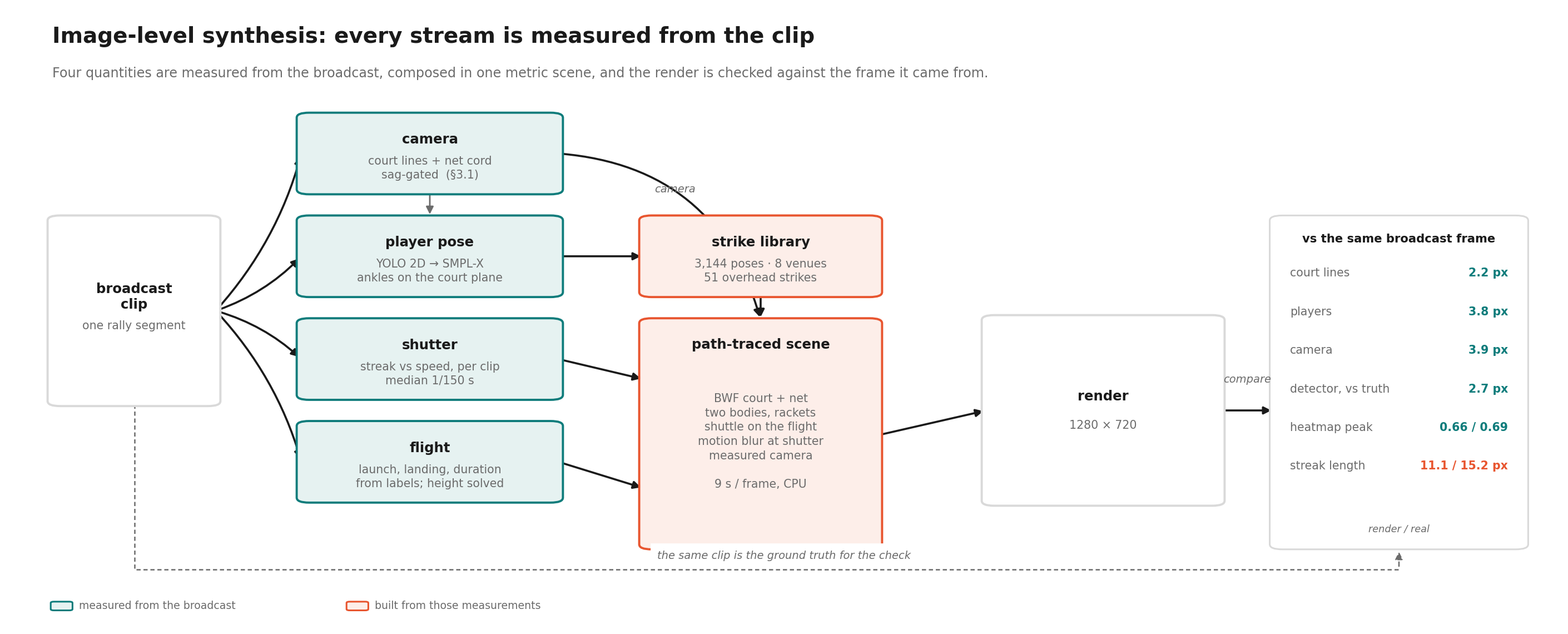
On 6,553 real tournament strokes, SimTrack3D recovers physically valid trajectories for 96.0% of strokes (with unfixable outliers explicitly flagged rather than hallucinated), compared to only 18.3% for unconstrained optimization baselines, reducing arrival endpoint error from 3.33 m to 0.60 m. We further extend the synthetic domain from trajectories to images: a broadcast-registered renderer whose camera, player poses and motion blur are all measured from the footage itself, agreeing with the frame it reconstructs to 2.2 px on the court lines and 3.8 px on the players, and on which a detector trained only on broadcast localises the shuttle to 2.7 px with the confidence it reports on real footage. Because it places a body fitted from the broadcast and a reconstructed shuttle in one metric frame, it also yields a geometrically independent probe of our own output: at 58 contact frames the striking wrist lies 0.52 m from the line of sight through the tracker’s own detection but 1.54 m from the reconstructed 3D point, localising the pipeline’s residual depth error to the stroke seam. Finally, we formulate an image-computable observability metric N, which exhibits a strict power-law correlation with the Cramér–Rao Lower Bound (CRLB ∝ N−0.98, R² = 0.83). This theoretical formulation quantifies the exact boundary where visual data ceases to constrain depth and the domain prior dominates.
1. Introduction
Deep heatmap regressors such as TrackNet[1, 2, 3] have established reliable 2D localization for small, high-speed sports projectiles. However, lifting these 2D pixel tracks into metric 3D trajectories remains an open challenge. Monocular 3D vision typically resolves depth ambiguity from object-centric cues: known physical dimensions, kinematic articulation, or surface texture gradients. In broadcast racket sports, every conventional cue collapses simultaneously:
- Absence of appearance scale. A tournament shuttlecock measures roughly 6.9 pixels in a 1280-pixel wide broadcast frame, elongating up to 17 pixels purely through motion blur. It possesses no resolvable texture, orientation, or metric extent.
- Degeneracy of motion parallax. Disambiguating depth along a viewing ray requires trajectory curvature induced by gravity and aerodynamic drag. Fast smashes traverse nearly collinear with the optical axis in just 10–15 frames at 30 fps; the subtle trajectory curvature is buried beneath visual tracking noise.
- Absence of planar ground bounces. Unlike tennis or table tennis[4, 5], where table bounces provide explicit geometric depth anchors, a shuttlecock flies strictly racket-to-racket, touching the court surface only to terminate the rally.
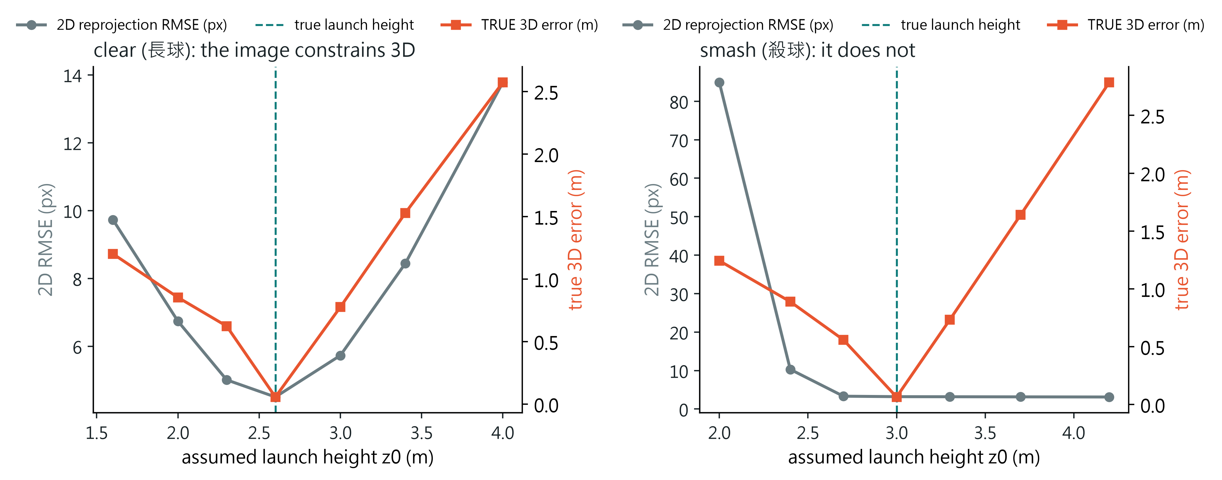
The reprojection fallacy. Because monocular sports broadcasts lack dense 3D ground truth, prior literature frequently validates reconstructions via 2D reprojection residuals or qualitative plausibility heuristics (e.g., net clearance or landing within the venue). As demonstrated in Figure 1, reprojection error is uninformative on high-speed strokes: on an axial smash, candidate trajectories exhibiting 3D errors from 0.06 m to 2.78 m yield virtually identical 2D residuals within 0.20 px. Validation by reprojection alone is structurally blind to massive line-of-sight depth errors.
Core intuition: anchoring depth to the floor. While a single broadcast view cannot resolve depth along a viewing ray directly, it resolves the ground plane with sub-pixel precision. Furthermore, every stroke in a rally is physically bounded by boundary conditions on this floor: the server's feet, the receiver's court positioning, the painted court lines, and the terminal landing. We formalize these spatiotemporal boundary conditions as planar anchors. The net cord provides the sole elevated, rigid metric reference above the floor.
In this work, we present SimTrack3D, a physics-grounded framework that recovers metric 3D projectile trajectories by exploiting non-coplanar net geometry, domain-faithful boundary-value simulation, and constrained null-space projection. Our core contributions are:
- Sag-gated non-coplanar calibration. We resolve the focal-length degeneracy of coplanar court lines by formulating a joint optimization over court lines and the elevated net cord, leveraging its physical 26 mm catenary sag as an independent validation gate to calibrate 32 broadcast venues.
- Aerodynamically feasible sim-to-real lifting. We introduce Shuttle3D, a ray-depth transformer trained on 77,728 synthetic flights generated by solving aerodynamic boundary-value problems (BVPs) over 13,010 real match events, achieving zero degradation on unseen camera setups.
- Null-space constrained rectification. We design a two-tier inference scheme that projects unconstrained proposals onto the physically admissible set along the two weakest eigenvectors of the reprojection curvature matrix J⊤J, eliminating physical violations without visual penalty.
- Observability theory and estimation bounds. We derive an image-computable observability metric, N, which exhibits a strict power-law scaling with the Cramér–Rao Lower Bound (CRLB ∝ N−0.98, R² = 0.83), formalizing the boundary where sensory data ends and domain priors dominate.
2. Related Work
2D projectile tracking in sports. Deep heatmap regressors typified by TrackNet[1] localise small, high-speed objects across temporal frame stacks. Subsequent iterations integrate trajectory rectification[2] and spatio-temporal attention[3], with parallel architectures adapted for soccer and table tennis. While motion blur is classically discarded as corruption, BlurBall[6] demonstrates that blur streaks encode instantaneous velocity vectors. In this paper, we leverage existing 2D detectors as observational front-ends and focus entirely on the ill-posed monocular 3D lifting problem.
Monocular 3D trajectory reconstruction. Reconstructing 3D trajectories from single-view footage requires strong priors to resolve depth ambiguities. MonoTrack[7] optimizes a single launch state per stroke against 2D detections via non-linear least squares. In table tennis, TT3D[4] and TT4D[5] exploit table impacts as metric boundary conditions. SynthNet[8] and Uplifting Table Tennis[9] demonstrate that transformers trained on synthetic arcs can learn monocular lifting. However, existing methods validate primarily on 2D reprojection or uncalibrated heuristics. We show that such proxies fail to penalize major depth degeneracies and introduce hard physical constraints to guarantee validity.
Sim-to-real transfer and system identification. Sim-to-real transfer paradigms span domain randomization[10], differentiable simulation, and domain adaptation. Rather than applying blind domain randomization over arbitrary camera distributions, our strategy follows rigorous system identification: we explicitly measure 32 broadcast camera geometries and synthesize trajectories from real match events.
Broadcast camera calibration and field registration. Planar field calibration from court markings provides an 8-DoF homography but leaves focal length entangled with extrinsic tilt and distance[11]. While vanishing-point estimators and deep registration networks[12][13] calibrate ground planes, sports fields lacking perpendicular vertical elements remain mathematically degenerate. We resolve this by incorporating the elevated net cord and its catenary profile into the calibration objective.
A longer survey, with the sim-to-real mechanisms and the constrained-estimation literature treated separately, is on the supplementary page.
3. Methodology
3.1 Sag-gated non-coplanar calibration
Let X = [X, Y, Z]⊤ denote a 3D coordinate in the canonical world frame, where the court surface lies on Z = 0. A planar homography relates court coordinates to image coordinates u = [u, v, 1]⊤:
Because court markings are strictly coplanar, H provides eight constraints, leaving focal length f and camera distance d mathematically degenerate. Evaluating Zhang's coplanar constraints[11] on our broadcast corpus reveals a 65% discrepancy in focal length estimates across plausible line correspondences.
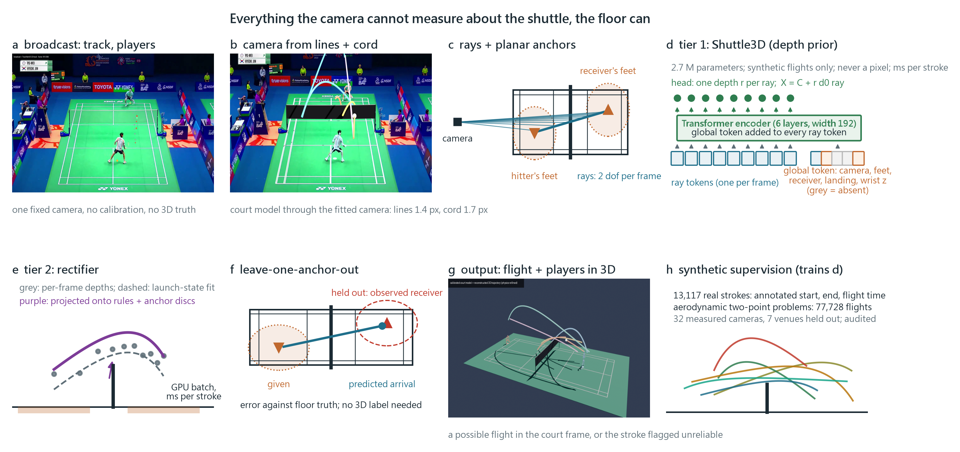
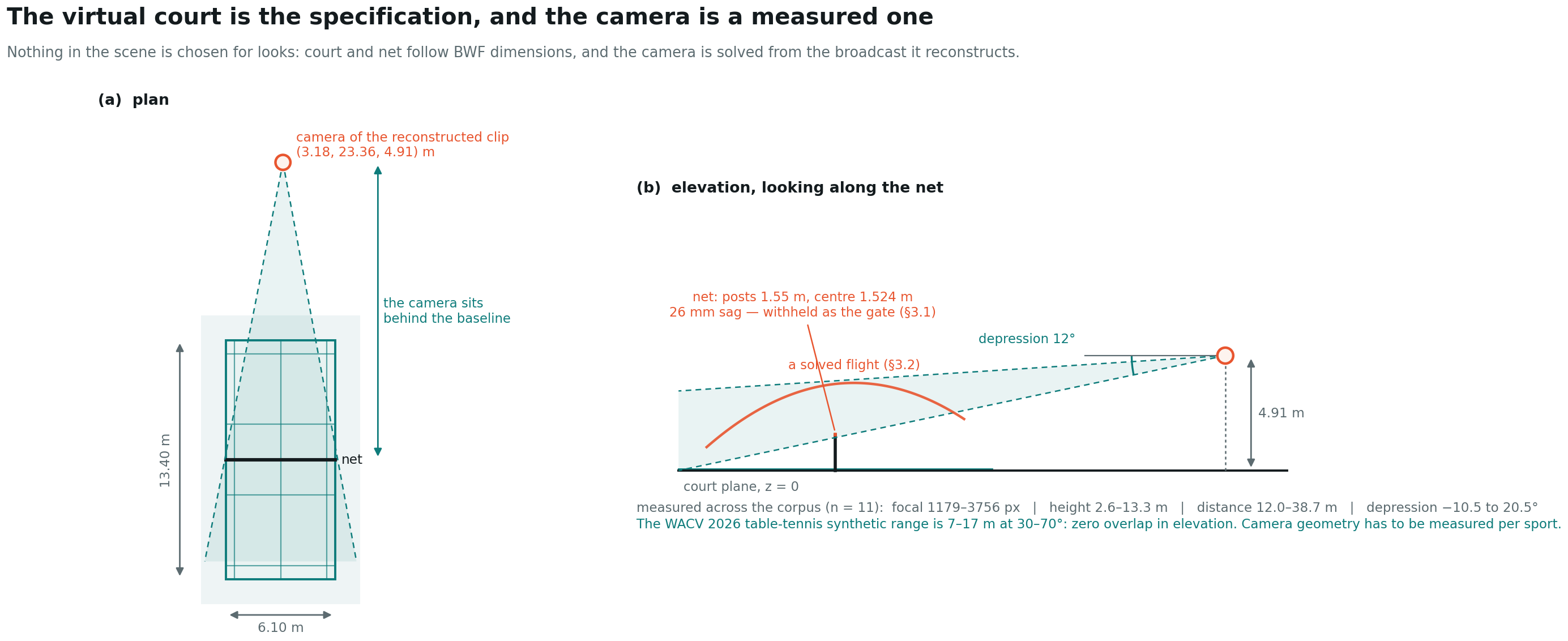
To decouple intrinsics from extrinsics, we incorporate the elevated badminton net cord. Under BWF specifications, the cord is suspended at post height Hp = 1.55 m and sags under gravity to Hc = 1.524 m at court center, representing an invariant vertical deflection of Δz = 26 mm across a width L = 6.10 m. In net-aligned coordinates, the cord profile follows a catenary:
Because Δz / L ≪ 1, the shallow catenary parabolic expansion holds:
Joint optimization. We extract sub-pixel court line segments and net-cord samples (e.g., 270 samples with 0.14 px fit residual on representative venues) via ridge filtering over temporal median backgrounds. We formulate calibration as a joint non-linear optimization over focal length f, rotation R, and translation t:
where d⊥ is the point-to-line orthogonal distance on the court plane, and π(·) denotes perspective projection of 3D net-cord points Qj.
Independent physical validation gate. The physical sag Δz is withheld from optimization. After convergence, we evaluate estimated vertical deflection, rejecting any calibration that violates our pre-defined physical tolerance:
This gate rejects degenerate minima where 2D line residuals appear optimal (<0.3 px) while camera distance is erroneous by several meters. Across 32 evaluated broadcast venues, 19 of 26 unannotated venues pass fully automatically (zero false passes, median corner error 0.033 m), and 22 pass with lightweight 4-corner initialization, exhibiting a median sag of 23.1 mm.
3.2 Aerodynamic boundary-value synthesis
A tournament shuttlecock experiences strong quadratic drag. With kinematic state s(t) = [x(t)⊤, v(t)⊤]⊤, the governing equations of motion are:
where g = [0, 0, −9.81]⊤ m/s2 and γ = g / vT2. With terminal velocity vT = 6.8 m/s, the aerodynamic drag parameter is γ ≈ 0.212 m−1.
Rather than sampling unconstrained launch states, we anchor synthesis to real tournament dynamics. Given annotated 2D court endpoints X0, XT and duration T from 13,010 match events in ShuttleSet, vertical trajectory reconstruction is formulated as a two-point boundary-value problem:
where launch and arrival heights Z0, ZT are drawn from stroke-specific priors. We solve for initial velocity v0 via a shooting method using a 4th-order Runge–Kutta integrator. At iteration k, with terminal residual Φ(v0) = x̂(T; v0) − xT, updates follow damped Newton steps:
The shooting solver achieves a 99.9% convergence rate.
Physical audit and feasibility filtering. In unconstrained synthetic generation, up to 10.6% of BVP solutions pass under the net cord (particularly on low-margin shots: 19.9% of net shots). To eliminate unphysical training data, we solve an ensemble of eight vertical height candidates per stroke, enforcing continuous-time physical criteria:
This yields 77,728 valid trajectory sequences. Continuous shooting enforces a strict 2 cm clearance margin, guaranteeing physical admissibility across the dataset.
3.3 Shuttle3D: ray-depth transformer
To achieve camera-agnostic generalisation, Shuttle3D operates on normalized viewing rays in world coordinates. For a 2D detection pt = [ut, vt]⊤, the unit viewing ray is:
where P is the calibrated camera matrix. Its intersection with the floor plane Z = 0 is:
where C is the optical center. Each frame is tokenized as a 7D feature vector: [rt⊤, Xfloor, Yfloor, 1horiz, t]⊤, where 1horiz flags near-horizontal rays where floor intersections diverge. The camera center is appended as a global conditioning token. A 6-layer Transformer encoder (dmodel = 192, 8 attention heads) estimates a relative depth dt along each ray:
where c0 is the court center. Estimating depth rather than absolute height prevents numerical divergence for low-angle views where rt,z → 0.
Domain-matched noise injection. To bridge the sim-to-real gap, training sequences are corrupted with empirically measured detector artifacts: heavy-tailed tracking noise (σ = 6.4 px median, 90th-percentile 24.6 px), burst dropouts, late visual acquisition, and calibration jitter. Differentiable hinge losses penalize violations of court boundaries and floor intersections during backpropagation.
3.4 Null-space constrained rectification
Because per-frame transformer predictions lack temporal coupling, raw trajectories exhibit high-frequency jitter and occasional physical violations. We therefore introduce a second-tier Rectifier. Given estimated 3D positions, we fit an initial 6D aerodynamic launch state s0 = [x0⊤, v0⊤]⊤ via non-linear least squares:
subject to hard court inequality constraints:
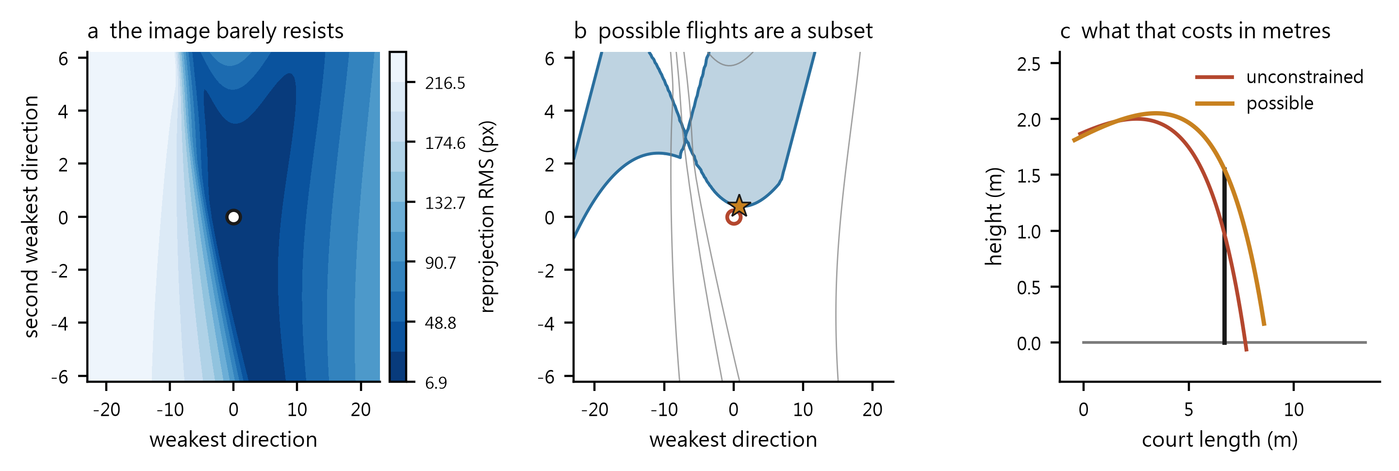
Projection along weakest observability directions. If the unconstrained fit violates any physical rule, the rectifier executes projected gradient descent. Critically, optimization steps are restricted to the 2D subspace spanned by the two eigenvectors [v5, v6] corresponding to the smallest eigenvalues of the Gauss–Newton reprojection curvature matrix J⊤J:
As illustrated in Figure 3, this subspace represents the line-of-sight depth degeneracy where metric adjustments cost negligible reprojection penalty. The optimizer operates under a maximum residual budget Δbudget = 14.0 px. In practice, the observed 90th-percentile reprojection cost on real tournament strokes is merely 0.76 px (median 0.00 px). Strokes that cannot satisfy all physical constraints within this budget are flagged as unreliable rather than forced into unphysical trajectories.
3.5 Spatiotemporal planar anchors
To ground the unobservable depth axis, we extract spatiotemporal boundary conditions directly from broadcast video:
- Hitter's ankle midpoint (t = 0). Extracted via 2D pose estimation; ankle midpoint is projected via H to define a horizontal launch disc (r = 2.5 m).
- Hitter's wrist elevation (t = 0). The hitting wrist viewing ray is intersected with the vertical plane passing through the hitter's feet, constraining launch height within a 1.0 m bound.
- Receiver's ankle midpoint (t = T). Ground position of the defending player at arrival, defining an arrival disc constraint (r = 2.5 m).
- Stationary landing spot (z = 0). On rally-final strokes, temporal clustering over stationary frames defines a terminal floor anchor (r = 0.5 m).
These anchors enter Shuttle3D as conditioning tokens and inform the Rectifier's optimization.
3.6 Image-level synthesis: a broadcast-registered renderer
The synthetic domain of §3.2 is a domain of trajectories: it transfers because the flight model and the camera distribution are measured, but it cannot exercise a detector, and it cannot tell us whether a reconstructed shuttle is where a human arm could have put it. We therefore extend the synthesis to images. The renderer places, in one metric frame, a measured broadcast camera, the court and net at BWF dimensions, two articulated human bodies, procedural rackets, and a shuttle on a flight from §3.2 — with motion blur at the shutter measured from the footage rather than assumed.
The renderer needs a rigid camera. For venues where §3.1 has run, its output is already one. Where a venue is described instead by four court corners plus a focal length, the projection P = [g1, g2, sKr3, g3] that keeps the Z = 0 slice exactly equal to the homography is pixel-exact on the court and not a physical camera: its decomposition returns negative focal lengths with det R = −1. Projection is insensitive to that mirror, so no estimation result is affected; a renderer handed it produces a black frame. The mirror is vertical in the image, and flipping the corresponding row of R recovers a proper camera whose reprojection agrees with the original to 3.92 px over nine points spanning the ground, the net-post tops, the players and the shuttle — inside the 6.03 px residual the corner annotations themselves carry.
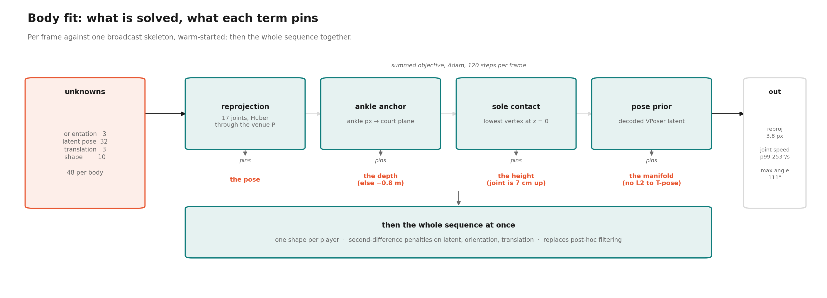
Players are fitted from the broadcast, not animated. No motion-capture corpus contains badminton, and a stock walk cycle would defeat the purpose. Instead an SMPL-X body is optimised per frame so that its joints project onto the 2D skeleton detected in that frame, through that venue's projection. Three constraints make the fit metric rather than merely plausible. Depth is anchored by back-projecting the ankle pixels onto the court plane — the same sub-pixel ground measurement the rest of this paper rests on — because apparent height is a poor depth cue and fixing the body to a nominal 1.72 m pulls both players about 0.8 m toward the camera; sole contact uses the lowest mesh vertex, not the ankle joint, which sits 7 cm off the floor; and the pose itself is the decoded 32-dimensional latent of a learned pose prior, so that only configurations a human can hold are reachable, with the whole sequence then refined jointly under acceleration penalties on the latent, the root orientation and the translation. The learned prior costs 1.3 px of reprojection against an L2 pull toward the rest pose (2.6 → 3.9 px) and buys poses that stay on the human manifold through lunges and low recoveries, where the L2 prior instead pays for pixels with implausible joint combinations.
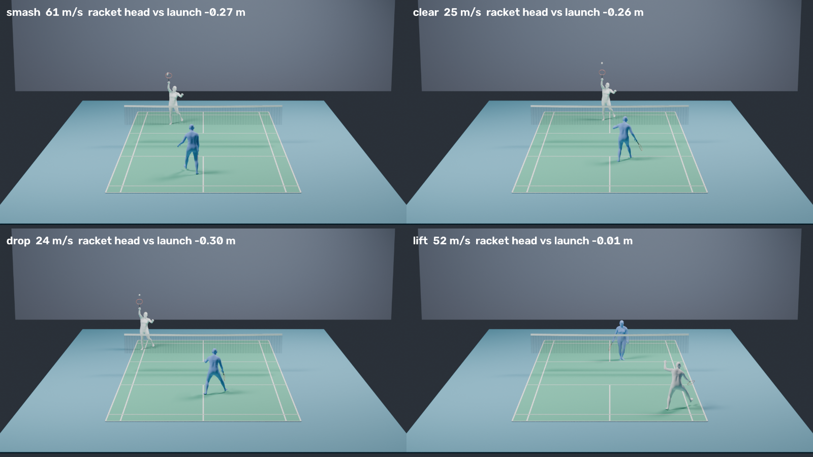
Strokes are populated from observed strikes. Fitting 16 clips across eight calibrated venues yields a library of 3,144 poses, each tagged with the racket hand, the wrist heights, and — from the stroke annotations — whether that frame is a contact and which player struck. To render a synthetic stroke, the striker is the observed striking pose whose racket head sits closest to the required launch height, yawed to face the net and translated so that the racket head coincides with the launch point and the feet rest on the floor. Launch point, landing point and duration come from the human annotations exactly as in §3.2; only the height between them is solved.
4. Observability and Estimation Bounds
4.1 Möbius projection of ballistic motion
Consider an unaccelerated path in 3D camera coordinates: Xc(t) = X0 + Vt. Under perspective projection, image coordinates follow:
Any constant-velocity 3D trajectory projects strictly as a 1D Möbius transformation of time parameterized by five degrees of freedom. Any visual deviation from this Möbius profile constitutes the empirical signature of physical acceleration.
4.2 The observability number N
We define the dimensionless observability number N as the root-mean-square deviation of the tracked 2D trajectory from the best-fit unaccelerated Möbius curve, normalized by detector noise σ2D:
The metric N computes the signal-to-noise ratio of observable acceleration directly from 2D pixel coordinates, requiring zero 3D ground truth. When N ≤ 1, trajectory bending is drowned in visual noise, rendering unconstrained monocular depth recovery mathematically indeterminate.
4.3 Fisher information and the Cramér–Rao bound
Under Gaussian observation noise, the Fisher Information Matrix over launch state s0 is:
For any unbiased estimator, covariance is bounded by Cov(ŝ0) ≽ I(s0)−1. Propagating to spatial position yields the Cramér–Rao Lower Bound on 3D variance:
Spectral analysis and dual degeneracy. SVD on I(s0) over 3,993 test strokes reveals that the right singular vector of σmin aligns with the camera ray to the launch point within a median angle of 1.9° (<10° on 89.0% of strokes), confirming that unobservability aligns with optical depth.
Crucially, the alignment angle to the line of sight and log N are uncorrelated (r = −0.00), while alignment angle explains only part of the conditioning (r = +0.35 with log σmin). This shows that monocular trajectory lifting exhibits two independent degeneracy mechanisms: (i) geometric collinearity with the viewing ray, and (ii) short temporal duration (small arc length). Grouping strokes by N accounts for both mechanisms simultaneously without requiring 3D truth.
4.4 Predicting recoverability and prior reliance
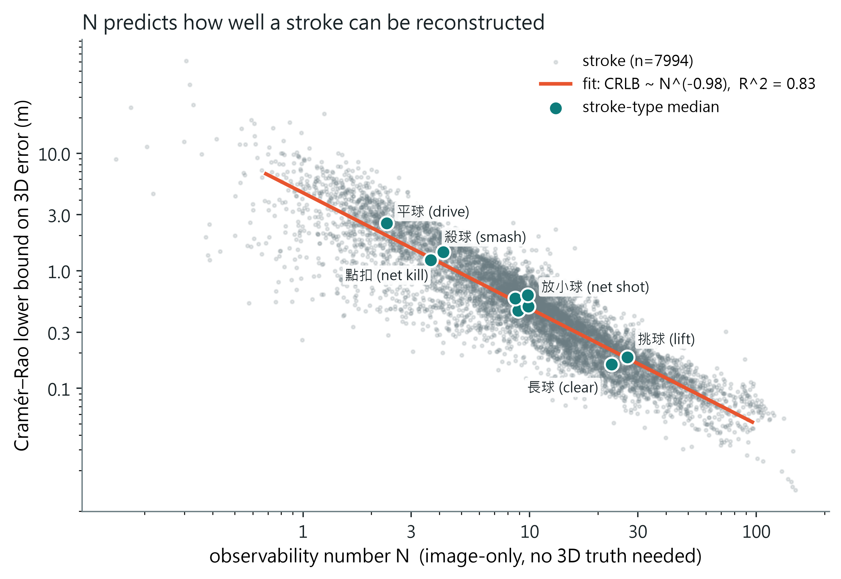
As plotted in Figure 8, across 7,994 anchored strokes, the observability metric N predicts the theoretical CRLB via an empirical power law:
Controlling for frame count, the partial correlation remains −0.59.
Quantifying prior reliance via bound violation. An unbiased estimator cannot outperform the CRLB. However, as shown in Table 1, Shuttle3D outperforms the unbiased CRLB on 9 out of 15 stroke categories (by up to 4.6× on flat drives). This occurs because our model acts as a Bayesian regularizer: on low-N strokes where visual evidence is indeterminate, it regresses toward typical tactical shot profiles, trading variance for domain-specific bias.
Significantly, the two types furthest above the bound — defensive lift (ratio 2.70) and clear (ratio 1.81) — possess high, prolonged arcs (N ≥ 14.9). Where visual evidence is strong, the model behaves as an honest estimator, paying the full unbiased variance price.
| Table 1 — Spectral conditioning, CRLB and error across all 15 stroke types (held-out synthetic strokes, n ≥ 30) | |||||
|---|---|---|---|---|---|
| Stroke type | Count | N | CRLB (m) | Shuttle3D (m) | Ratio |
| Lift | 2,325 | 27.0 | 0.183 | 0.271 | 1.48 |
| Clear | 894 | 23.0 | 0.160 | 0.289 | 1.81 |
| Cross-net | 200 | 15.3 | 0.287 | 0.438 | 1.53 |
| Defensive lift | 144 | 14.9 | 0.303 | 0.819 | 2.70 |
| Over-cut drop | 78 | 11.1 | 0.424 | 0.444 | 1.05 |
| Push | 311 | 9.9 | 0.497 | 0.400 | 0.80 |
| Net shot | 2,665 | 9.8 | 0.619 | 0.398 | 0.64 |
| Drop | 948 | 8.9 | 0.458 | 0.390 | 0.85 |
| Block | 1,518 | 8.6 | 0.583 | 0.542 | 0.93 |
| Defensive drive | 149 | 6.3 | 0.723 | 0.787 | 1.09 |
| Tap smash | 390 | 4.2 | 1.440 | 0.400 | 0.28 |
| Rear drive | 228 | 4.0 | 1.059 | 0.645 | 0.61 |
| Smash | 1,381 | 3.7 | 1.232 | 0.344 | 0.28 |
| Rush | 176 | 3.2 | 1.886 | 1.147 | 0.61 |
| Drive | 240 | 2.3 | 2.539 | 0.556 | 0.22 |
5. Experiments and Results
5.1 Experimental setup
Datasets. We evaluate across two corpora. The ShuttleSet benchmark supplies 6,553 tournament strokes across 10 venues featuring annotated player ground locations and TrackNetV3 detections. The TrackNetV3 broadcast corpus supplies 2,592 interior strokes from 22 international tournament venues with frame-level 2D ground truth, calibrated purely from broadcast video via our non-coplanar pipeline.
Evaluation metrics. For synthetic data, we report per-frame median 3D error. For real footage devoid of dense 3D ground truth, we evaluate: (i) physical feasibility rate, the percentage of strokes satisfying all court, net and floor constraints; (ii) reprojection cost, the pixel penalty incurred by constrained projection; and (iii) leave-one-anchor-out error, the metric discrepancy between predicted trajectory boundaries and held-out physical floor positions.
5.2 Baseline comparisons
We benchmark against state-of-the-art monocular projectile reconstructors and classical estimators. MonoTrack[7] optimizes a per-shot launch state and drag coefficient under unconstrained reprojection loss. Iterated EKF + RTS smoother combines extended Kalman filtering with Rauch–Tung–Striebel backwards smoothing over identical aerodynamic models. Batch MAP performs global maximum a posteriori optimization over the complete temporal frame sequence.
| Table 2 — Quantitative baseline comparison on matched real and synthetic sets. 400 synthetic test strokes and an identical benchmark subset of 1,138 real tournament strokes. On the full 6,553 real corpus, SimTrack3D achieves 96.0% feasibility, 0.91 m launch error and 0.60 m arrival error. | ||||
|---|---|---|---|---|
| Method | Synth 3D (m) | Real valid | Launch err (m) | Arrival err (m) |
| MonoTrack | 1.001 | 18.3% | 2.81 | 3.33 |
| EKF + RTS smoother | 1.383 | 12.5% | 6.85 | 3.09 |
| Iterated EKF | 0.323 | 22.1% | 3.27 | 2.65 |
| Batch MAP | 0.317 | 22.4% | 2.95 | 2.55 |
| Ours (Shuttle3D + rectifier) | 0.314 | 97.4% | 1.00 | 0.57 |
As reported in Table 2, unconstrained optimization baselines fail catastrophically on real tournament footage: MonoTrack yields physically plausible flights on only 18.3% of strokes, with arrival endpoints missing the defending player by a median of 3.33 m.
Crucially, Batch MAP outperforms Shuttle3D on the two highest-N stroke types where sensory evidence is rich (lift: 0.136 m vs. 0.279 m; clear: 0.139 m vs. 0.309 m). This directly corroborates our theoretical prediction: an efficient unbiased estimator attains the CRLB when sensory information is uncompromised. However, on fast smashes where N collapses, Batch MAP deteriorates severely (1.264 m vs. 0.229 m for Shuttle3D), achieving only 22.4% valid flights on real footage. In contrast, SimTrack3D delivers 97.4% physical feasibility on this benchmark subset, achieving an arrival error of 0.57 m.
5.3 Ablation: input space parameterization
To evaluate whether performance gains stem from model capacity or geometric parameterization, we evaluate four input representations under identical Transformer backbones and training schedules on held-out strokes: world rays to depth along the ray (ours), world rays to 3D coordinates, pixels plus the camera matrix to 3D coordinates, and pixels plus a learned camera embedding to 3D coordinates.
| Table 3 — Impact of input space parameterization. Held-out strokes viewed through seen vs. held-out camera configurations; median 3D error in metres. | |||
|---|---|---|---|
| Representation | Seen cams | Unseen cams | Out-of-ray (m) |
| Ours (ray → depth) | 0.388 | 0.387 | 0.000 |
| Ray → 3D position | 0.371 | 0.406 | 0.059 |
| Pixels + camera matrix | 0.338 | 0.579 | 0.215 |
| Pixels + intrinsics/center | 0.341 | 0.690 | 0.464 |
| Pixels + learned embedding | 0.329 | 1.408 | 0.934 |
As shown in Table 3, pixel-space baselines perform well on seen cameras by memorizing venue-specific depth priors, but degrade severely (1.7× to 4.3×) when evaluated on novel camera setups. In contrast, our ray-depth formulation achieves zero performance degradation on unseen cameras (0.388 m vs. 0.387 m), confirming robust geometric transfer.
5.4 Leave-one-anchor-out real-world validation
Because real footage lacks dense 3D ground truth, we validate physical accuracy by holding out each spatiotemporal anchor in turn and measuring prediction discrepancy against real floor positions.
| Table 4 — Leave-one-anchor-out evaluation on 6,553 real strokes. Discrepancy measured against held-out player ground positions. All configurations use the same model and the same one-step rectifier as Table 2. | |||
|---|---|---|---|
| Anchor configuration | Valid | Launch err (m) | Arrival err (m) |
| No anchors | 96.0% | 0.91 | 0.60 |
| w/o hitter feet | 84.5% | 0.72 | 0.50 |
| w/o receiver feet (n = 5,747) | 93.7% | 0.69 | 0.55 |
| w/o landing (n = 530) | 69.2% | 1.33 | — |
| All anchors enabled | 80.1% | 0.68 | 0.48 |
Table 4 demonstrates that planar floor anchors systematically reduce boundary endpoint error. Enforcing all anchors as strict hard inequalities during rectification reduces overall feasibility to 80.1%, reflecting noise in visual pose detections. Consequently, our final pipeline treats anchors as soft tokens in Tier 1 and reserves hard constraints in Tier 2 strictly for court boundary rules.
5.5 Diagnostic: net-cord clearance boundary
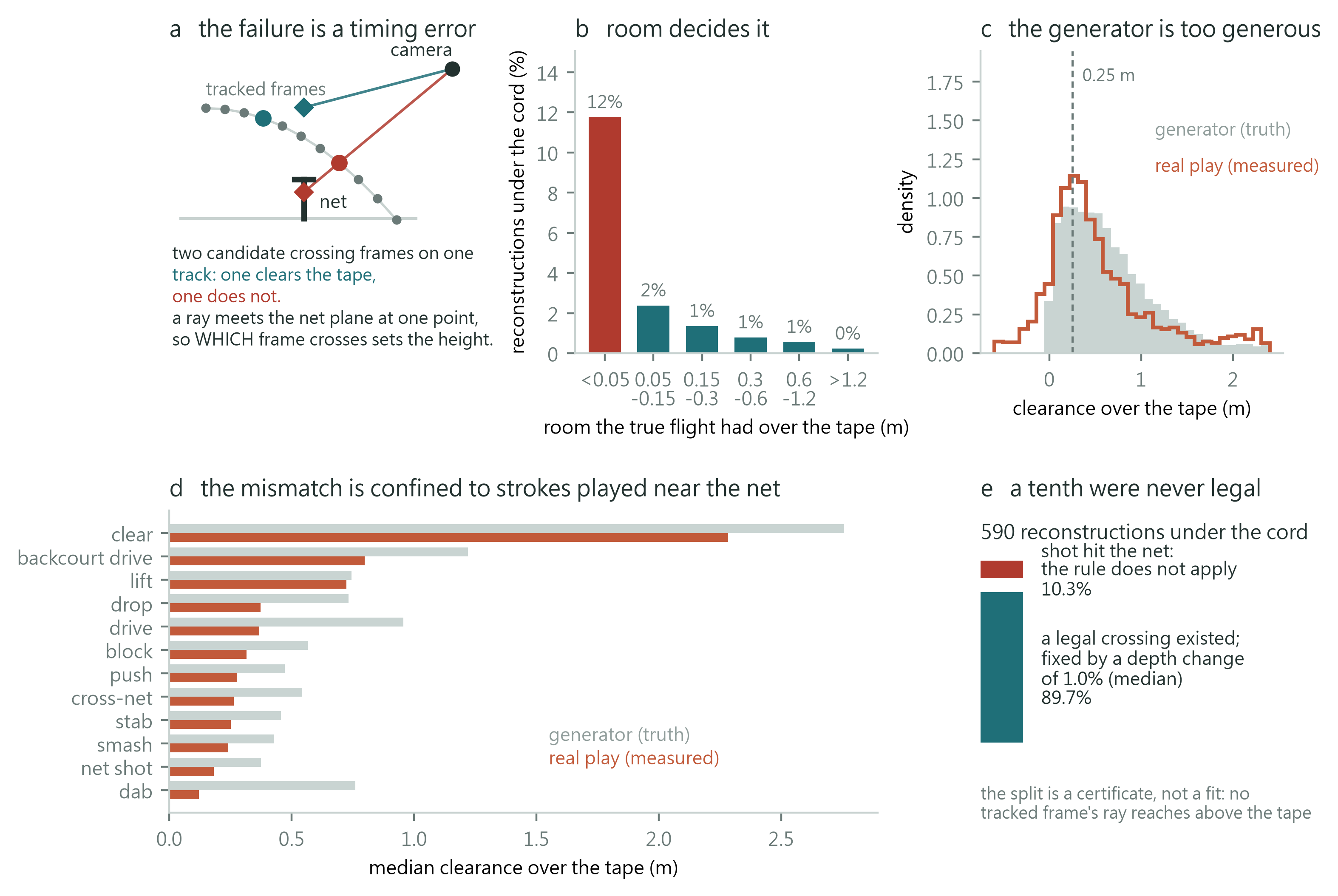
As illustrated in Figure 9, on real footage 8.9% of unconstrained reconstructions violate net clearance. Our diagnostic confirms that this is not an altitude estimation failure.
- Timing vs. height error. An image ray intersects the known net plane at exactly one height; clearance is determined solely by the estimated frame of net crossing.
- Boundary sensitivity. 89.7% of cord violations are resolved by a uniform depth scaling of merely 1.0% (median shortfall 0.11 m). Net clearance is a high-sensitivity boundary test decided at the third significant figure of depth.
- Real vs. synthetic margin. In tournament play, real players execute net shots clearing the tape by a median of 0.18 m, whereas synthetic BVP generators produce clearances averaging 0.37 m.
- Net-hit trajectories. A ray-plane certificate reveals that 10.3% of apparent violations could not clear the tape at any depth; these represent shots terminating in the net, where the clearance rule is inapplicable.
5.6 Ablation analysis
| Table 5 — Component progression and synthesis ablation. Raw network feasibility vs. rectifier return rate, alongside a training-synthesis comparison on 800 real strokes. | |||
|---|---|---|---|
| System stage | Raw valid | Return valid | Arrival (m) |
| Shuttle3D (clean 2 px noise) | 78.9% | — | 0.73 |
| + measured noise model | 85.0% | — | 0.59 |
| + court rule losses | 88.4% | — | 0.60 |
| + Tier-2 rectifier | — | 96.0% | 0.60 |
| Synthesis comparison (800 real strokes): | |||
| Random launch state sampling | 67.9% | — | 1.29 |
| BVP anchored synthesis (ours) | 64.6% | — | 0.90 |
Table 5 delineates the progression across stages. Incorporating measured tracking noise and rule losses improves raw network validity from 78.9% to 88.4%. The Tier-2 rectifier establishes a 96.0% final return rate of physically valid trajectories on real tournament matches.
Crucially, the synthesis ablation highlights that physical feasibility does not imply metric accuracy: random launch parameter sampling achieves a higher raw feasibility rate (67.9% vs. 64.6%) by generating conservative, high-clearance arcs, but suffers severe metric degradation on real strokes (1.29 m vs. 0.90 m endpoint error).
5.7 How close the rendered images are to broadcast
A synthetic image domain is only worth building if it is close to the real one, so we measure the distance rather than assert it. We reconstruct one real rally segment in full — same camera, both players fitted per frame from that footage, shuttle on the reconstructed trajectory — and compare the render against the broadcast frame it was built from.
| registration of the rendered twin to the broadcast frame | value |
|---|---|
| court lines, 1,440 samples over 12 lines | 2.2 px median (p90 6.0) |
| near / far player, 91-frame sequence fit | 3.9 / 3.8 px median |
| rendering camera against the venue projection | 3.9 px, worst of 9 test points |
| camera motion within a rally (phase correlation, 20 frames) | 0.25 px median |
| shuttle streak, rendered vs real (53 annotated frames) | 11.1 px vs 15.2 px major axis |
| render cost | 9 s/frame, CPU path tracing, 1280×720 |
Court alignment lands at the residual the corner annotations themselves carry, and the fitted bodies sit within the detector's own keypoint noise. The one clear shortfall is streak length. The minor axis matches (6.1 against 5.4 px), so the shuttle's size is right and only the exposure is short: the render used the corpus-median shutter of 1/116 s while this clip is slower. Shutter is measurable per clip from the streaks themselves — median 1/150 s with an eight-fold spread across clips, 1/91 to 1/1708 — and wiring that per-clip value into the renderer is the obvious correction.
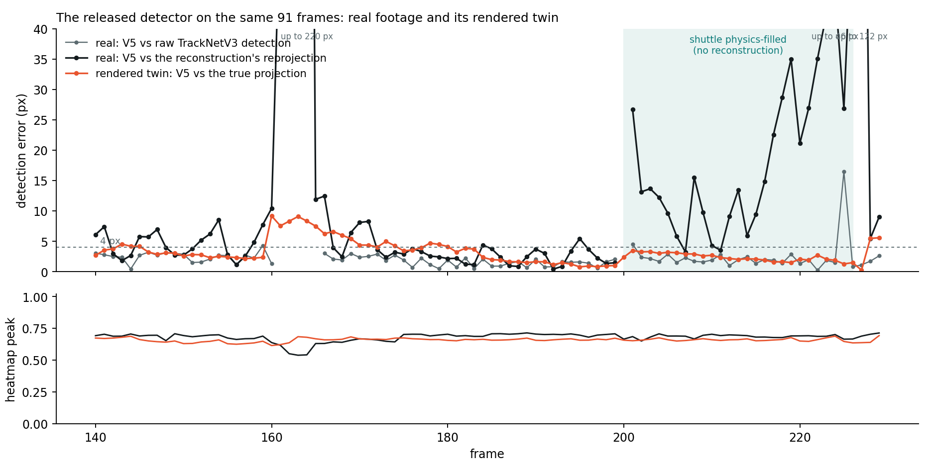
The acceptance test: a detector that has never seen a render. Registration says the geometry is right; it does not say a detector would treat the image as broadcast. So the released TrackNetV5-Lite — trained on real footage only, not fine-tuned here — is run on the 91 rendered frames and on the 91 real frames they reconstruct, and scored against the projected 3D on the render. On the real side this corpus has no human per-frame 2D; the two references available are the raw TrackNetV3 detection (another detector's opinion) and the reconstruction's own reprojection (which carries the reconstruction's error), and both are reported as what they are.
| the released detector, same 90 frames | reference | median | p90 | < 4 px | < 8 px | heatmap peak |
|---|---|---|---|---|---|---|
| real footage | raw TrackNetV3 detection | 1.9 px | 3.0 | 96% | 99% | 0.69 |
| real footage, clean strokes | reconstruction reprojection | 3.5 px | 10.6 | 63% | 83% | 0.69 |
| rendered twin | true projection | 2.7 px | 5.6 | 74% | 96% | 0.66 |
A detector that has never seen a rendered pixel localises the rendered shuttle to 2.7 px at the median with 96% of frames inside 8 px, and reports the same heatmap confidence on the render as on the broadcast (0.66 against 0.69). The only rendered frames it misses by more than 8 px are the contact frames 160–164, where the racket frame occludes the shuttle at 8–9 px; the physics-filled frames, with no player near the shuttle, are its best (2.2 px). What this does not establish is that it fails on the same frames as on real footage: the real side has no ground truth, so a per-frame comparison is a comparison of two detectors, and we do not draw one.
The population step has its own failure mode, and it is a sampling failure rather than a fitting one. A first library built from randomly chosen 100-frame windows contained exactly one overhead strike among 58 striking poses, which makes a synthetic smash impossible to stage. Two explanations were natural and both were tested and rejected: keypoint confidence at overhead contacts is the highest in the corpus (0.97 against 0.94 elsewhere) and the fitted wrist reprojects 5.5 px from the detected one, so the fit follows the data; and the distance from the nearest fitted wrist to the line of sight through the raw detection, swept around each contact, reads 1.08 / 0.74 / 0.52 / 0.66 / 0.95 m at −8 / −4 / 0 / +4 / +8 frames — a clean minimum exactly at contact, so the striker is identified correctly. The cause is that random windows are mostly footwork. Selecting windows by the annotated stroke class, since smash, clear, cut and push are struck above the head, changes the library without changing a line of the fitter.
| pose library, 16 clips over 8 venues | random windows | selected by stroke class |
|---|---|---|
| striking poses | 58 | 66 |
| overhead-class strikes | 1 | 51 |
| highest reachable racket head | 1.69 m | 2.24 m |
| racket head vs required launch point, overhead strokes | 0.80 m | 0.26–0.30 m |
5.8 An independent check on contact-frame depth
Placing a fitted body and a reconstructed shuttle in the same metric frame creates a comparison this problem does not otherwise admit, and it bears directly on the wrist-elevation anchor of §3.5. The reference pixel is the tracker’s raw detection, which the reconstruction consumes but never edits; nothing in the pose fitting sees a shuttle at all, and the body’s depth comes from ankles on the court plane. The two sides of the comparison are therefore independent of each other and of the reconstruction being tested.
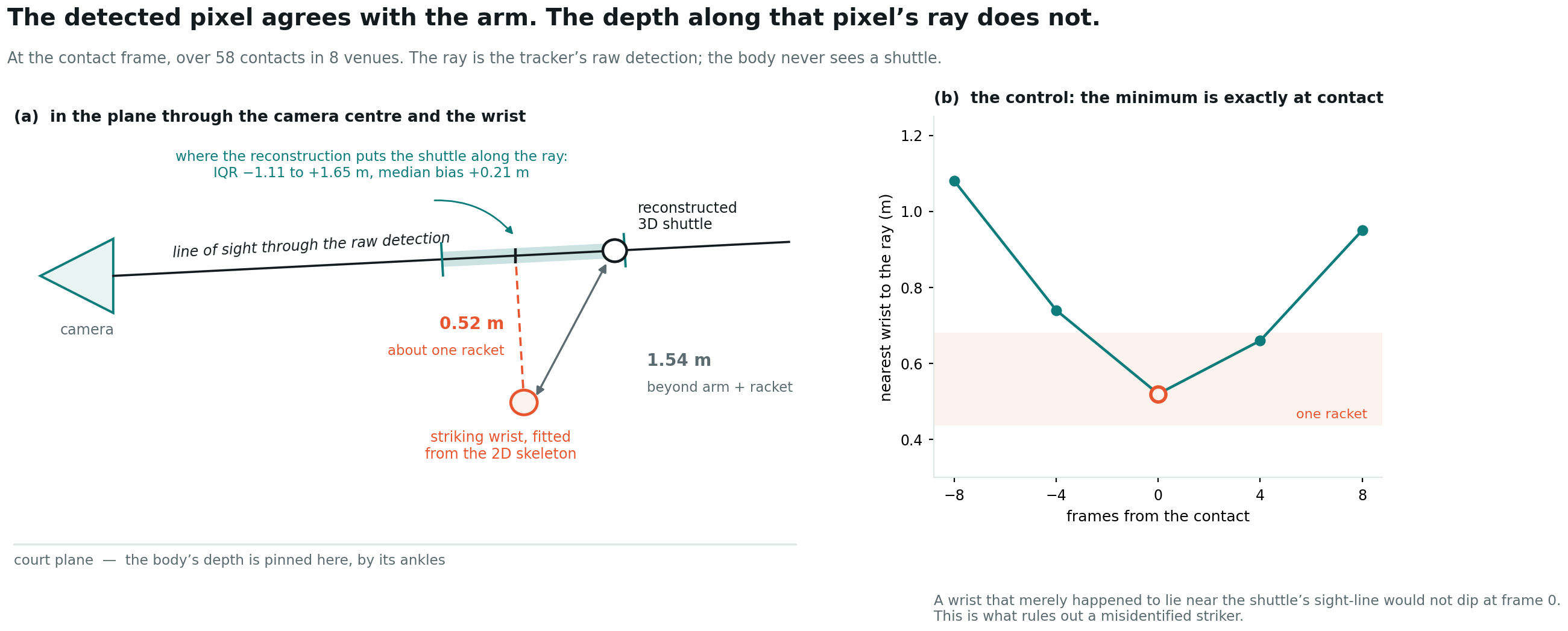
Over 58 contact frames in 8 venues, the distance from the striking wrist to the reconstructed 3D shuttle is 1.54 m — beyond an arm plus a racket — while the distance from the same wrist to the line of sight through the raw detection is 0.52 m, which is about one racket. The detection therefore agrees with the fitted body, and the depth along that ray is what disagrees. The reconstructed point itself sits only 0.09 m off the detection’s ray, so the 2D fit is tight; resolved along the ray, its depth is scattered with a slight far bias: a median 0.21 m beyond the wrist’s closest approach, with an interquartile range of −1.11 to +1.65 m.
This is what §4 predicts rather than a contradiction of it. The contact frame is the seam between two solved flights, the instant at which the arc being fitted ends and the next begins, and it carries the least depth information of any frame in the stroke. The measurement turns that qualitative statement into a number, on 58 events rather than the 14 rally-final anchors of §5.4, and it says that reported depth at the moment of impact should carry an explicit uncertainty of roughly a metre while the same trajectory's mid-flight depth does not.
6. Discussion and Limitations
Operational scope and tracking continuity. Following standard broadcast sports vision pipelines[7], our framework operates under the operational assumption of a stationary main broadcast camera. Furthermore, trajectory lifting is performed on stroke intervals with at least 45% visual tracking continuity. Across tournament venues, raw detector recall ranges from 9% to 92%, meaning analyzed rallies naturally reflect trackable game segments.
Aerodynamic model sensitivity. Synthesis and estimation share a quadratic drag model with terminal velocity vT = 6.8 m/s. To quantify sensitivity to drag misspecification, we evaluated the estimator under perturbed terminal velocities (vT ± 15%). Perturbing vT by −15% (5.78 m/s) increases mean 3D error by 63% (0.471 m → 0.769 m) and launch error from 0.309 m to 1.474 m. Remarkably, physical feasibility remains virtually unchanged (98.7% → 96.5%). This reinforces our core thesis: physical plausibility provides a necessary sanity boundary, but does not guarantee metric accuracy.
Ground truth in broadcast sports. Monocular sports vision lacks large-scale 3D sensor ground truth. In our corpus, 14 rally-final strokes provide an exact physical 3D anchor (z = 0 at landing), on which SimTrack3D achieves a median 3D error of 1.00 m and a landing height error of 0.32 m. While these 14 strokes serve as an absolute sanity check rather than a comprehensive benchmark, our leave-one-anchor-out formulation provides a scalable proxy for single-camera sports evaluation. §5.8 adds a second, geometrically independent probe of the same kind: a human body fitted from the broadcast, which never sees a shuttle, bounds where the striking hand was at 58 contact frames and localises the pipeline’s weakest depth to the stroke seam.
What the image-level domain does not yet establish. §3.6 renders images that register to broadcast at 2.2 px on the court and 3.8 px on the players, and §5.7 shows a detector trained only on broadcast treats them as broadcast — 2.7 px median against the true projection, with the same confidence. What has not been run is the converse: a detector trained on the renders and evaluated on real footage. Until it is, the renderer is validated as a measurement instrument and as an evaluation domain, not yet as training data. Its known gaps are the shutter (per-clip exposure is measured but not wired in), lighting estimated from the real shadows, and the absence of crowd, stands and clothing.
7. Conclusion
We presented SimTrack3D, a principled framework for monocular 3D trajectory reconstruction of fast-moving sports projectiles from broadcast video. By resolving focal-length degeneracy via sag-gated net-cord calibration, synthesizing domain-faithful trajectories via aerodynamic BVP formulation, and enforcing physical rules along unobservable null-space directions, SimTrack3D achieves 96.0% physically valid reconstructions on real tournament matches. Furthermore, our observability theory formalizes the boundary where sensory data ends and domain priors take over, establishing a rigorous foundation for single-camera 3D trajectory estimation.
Interactive 3D model
The calibrated court, net, broadcast camera frustum and forty reconstructed trajectories, exported from Blender. Drag to orbit, scroll to zoom.
BibTeX
@misc{chang2026shuttle3d,
  title  = {SimTrack3D: Monocular 3D Trajectory Prediction of Fast-Moving
            Shuttlecocks via Broadcast-Calibrated Sim-to-Real Transfer},
  author = {Chang, Gino},
  year   = {2026},
  note   = {Project page}
}
Court and net geometry follow BWF specifications (6.10 × 13.40 m doubles court; net 1.55 m at the posts, 1.524 m at centre). Shuttle flight model: quadratic drag with 6.8 m/s terminal velocity, RK4. Tracking: TrackNetV3. Rendering: Blender 4.2. Every ordinary number on this page comes from the experiment logs of this project.